
HEALTH ECONOMICS
Mean statistics can be nice: Using normal techniques when data are not normal

Jeffrey S. Hoch, PhD
Carolyn S. Dewa, MPH, PhD
In this ninth article in the health economics series, we explore when simple methods assuming normal distributions can be used to analyze skewed data, such as costs or outcomes. Skewness occurs because many people described by the data have low (or high) values but there are also some extreme observations, resulting in a data distribution that is neither “normal” nor symmetrical. In such circumstances, some may worry about whether the simple average (the mean) may be biased and if simple tests of it (e.g., the t test) may not apply. We provide examples illustrating these scenarios and explain how the sample mean is unbiased regardless of how the data look. In addition, we explore how the central limit theorem ensures that the simple t test is an acceptable choice in many scenarios.
KEY WORDS: leadership, simple statistics, health economics
Hoch JS, Dewa CS. Mean statistics can be nice: using normal techniques when data are not normal. Can J Physician Leadersh 12(3): 150-157. https://doi.org/10.37964/cr24813.
Evidence informing health care leaders’ decisions may come from data that do not show a “normal” (i.e., bell-shaped) distribution. For example, you might need the average cost from a skewed cost-distribution or the expected value from a satisfaction survey where most answers gravitate to the upper (or lower) part of the response range. You might recall the sacrosanctity of the normal distribution from classes, with the sample mean and simple tests (e.g., a t test) helping to inform strategic leadership decisions. But, they can only do that if the data are normally distributed, right? This article discusses why and when skewness is not an impediment to using the sample mean and analyzing it with common statistical tests.
When data have different shapes
The shape of your data’s distribution reflects its key characteristics. For example, cost data have a lower limit of $0 and usually a long tail to the right because of some high-cost patients. Treating a few long-stay or high-expense patients produces the familiar “small-proportion-of-patients-drive-most-cost” pattern often observed in health care data. When Le and colleagues1 studied the cost of dizziness, they identified over 12,000 cases in a Canadian tertiary care hospital’s data between January 2009 and December 2014. The authors noted that the cost data were highly skewed in spite of the large sample. Enlarging the sample does not eliminate skewness, as the existence of a small group of extremely costly individuals does not diminish with increased sample size. The authors used the mean costs in their data to estimate the cost of dizziness across all of Ontario by multiplying the mean cost by the relevant number of people. Given that the data were skewed, is the estimate of the mean biased?
Data can be skewed in the other direction because of “ceiling” effects. Ceiling effects occur when there is a fixed upper limit (e.g., 100 on a scale from 0 to 100) and most people are at or near that upper limit. A familiar example is patient satisfaction ratings. For patient satisfaction, the EQS-H scale (Échelle de Qualité des Soins en Hospitalisation) has been used to assess inpatient satisfaction with medical information and relationships with staff,2,3 and, although the EQS-H is convenient to use for both hospitals and patients, its psychometric properties are compromised by, among other things, ceiling effects.4 If most patients who complete satisfaction studies are generally highly satisfied (or unsatisfied), a large clumping of scores will occur at the top (or bottom) of the scale. Does the skewness of these data prevent their use to explore areas for quality improvement? For example, could a simple t test be used on the skewed data to determine whether a quality improvement initiative is associated with a significant improvement in scores?
What about data that are U-shaped, with peaks at both low and high ends of the distribution? This pattern has been observed in physician satisfaction and burnout studies. A study published in the Mayo Clinic Proceedings reported that professional challenges for physicians vary by career stage, with mid-career appearing to be a particularly challenging time.5 The authors suggested that their findings about mid-career challenges are, “consistent with the Community Tracking Study of physicians conducted in the 1990s6 and with studies conducted in other fields.7” If you believe the authors’ claim that, “the nadir in satisfaction during middle career is not a new phenomenon, [and it is] unlikely that the findings… are due to generational effects alone,” then your organization’s survey of physician satisfaction may produce data that are U-shaped. Will you be able to test if your organization is different from the national average using a t test?
Q: Is the sample mean biased? A: No.
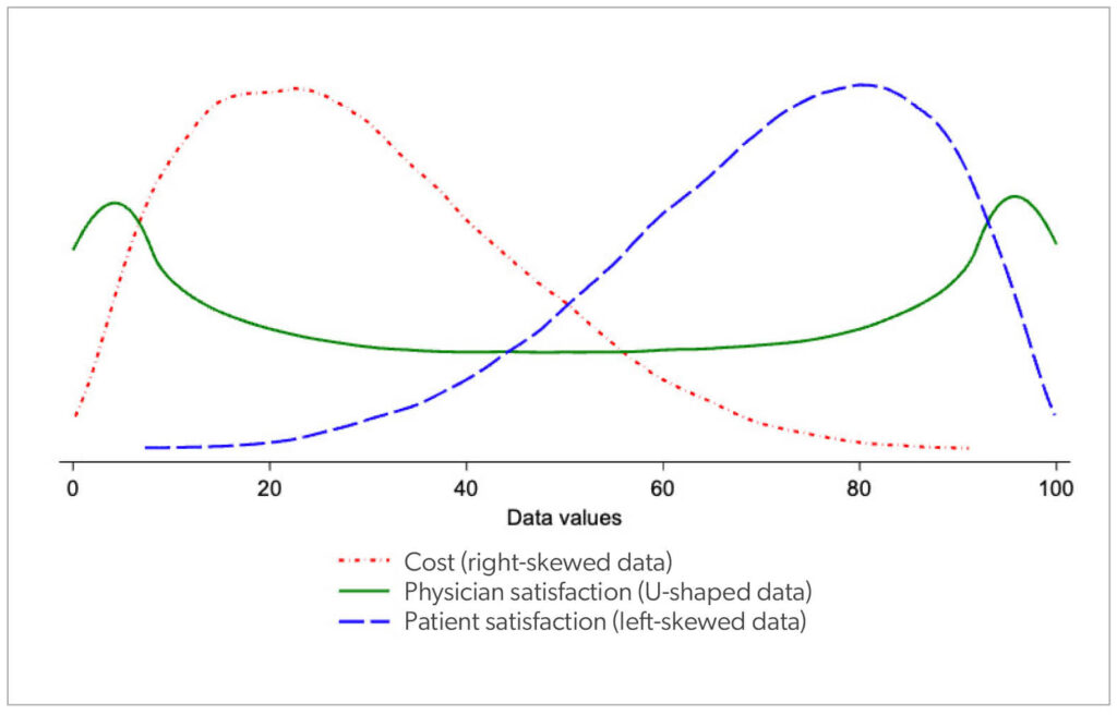
Figure 1 shows the data distributions of the three variables described above: cost, physician satisfaction, and patient satisfaction. Each shape differs from the standard normal distribution. Nevertheless, the sample average is not a biased estimate of the mean. To the contrary, the sample average is the best linear unbiased estimate.8 In the appendix, we explain this in more detail. The main point is that, according to theory, the sample mean is unbiased for all distributions, including skewed data.
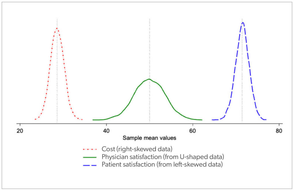
Empirically, we can double-check this by taking lots of samples from the data distributions in Figure 1 and calculating the mean of each sample. Figure 2 shows what happens if we make a graph of all the means we calculate from all the samples we take. There are two essential observations.
First, the dotted vertical lines in Figure 2 are the mean values from the distributions in Figure 1. One can see that the distributions of the means of each sample collect around the same expected value as the data (the peaks in Figure 2 are at the mean values of Figure 1’s distributions, shown with vertical lines in Figure 2). This is empirical proof that, regardless of the shape of the data’s distribution, the mean’s distribution will centre on the data’s expected value. This illustrates the claim that the mean is unbiased.
Q: Are statistical tests that assume normality wrong? A: Not really.
The second observation from Figure 2 involves the shapes of the distributions of the means. Each distribution in Figure 2 is bell-shaped (they all have the shape expected of a normal distribution). The left-most normal distribution in Figure 2 (cost) is a collection of means fashioned together from repeated samples of the right-skewed data shown on the left in Figure 1. Likewise, the right-most normal distribution in Figure 2 (patient satisfaction) is a collection of means fashioned together from repeated samples of the left-skewed data on the right in Figure 1. Regardless of the shape of the data, the distribution of the means is bell-shaped. This finding is not surprising; it is formally described by the Central Limit Theorem, which some have called the “most fundamental theory in modern statistics.”9 However, it is important to note that, when applying the theorem, the bigger the skewness in your data, the bigger your sample needs to be to assume the mean is normally distributed.
In our example, Figure 2 is made from lots of samples from people (n = 100). With this relatively small sample size, the mean is able to overcome the non-normality of the data distributions in Figure 1. For statistical testing, if you are willing to assume the sample mean for your data is normally distributed, then you can use the t test for 95% confidence intervals and statistical tests. With data that are not very skewed, n > 30 is a rule of thumb where assumptions about the data distribution no longer matter, since the sampling distribution for the mean is considered normal, according to the Central Limit Theorem.9 This means that in many circumstances, statistical tests that assume normality (e.g., the t test for means) are not incorrect, even if the data are skewed. The appendix has more about the Central Limit Theorem.
Worst case scenario (large skew, small sample size)
With some data (e.g., cost or charges), often there is no theoretical upper bound and this can lead to data distributions with tremendous skewness and major deviations from normality. A small sample size leads to legitimate concern that the Central Limit Theorem may not hold. What should one do then? In the article, “Help, my data are skewed,” Dr Alice Sitch recommends either transforming the data or conducting non-parametric tests (not assuming normality).10
But these alternatives are not without problems of their own. For example, while a transformation may create data that are normally distributed on the transformed scale, the inferences will be about the data on the transformed scale. This can make the interpretation of statistical tests difficult. A common transformation for skewed cost data is the log transformation, e.g., transformed cost = log(cost). A t test of log costs will provide information about whether log costs differ; leaders may care more about actual costs. Retransformation back from log cost to actual cost is not straightforward. Moreover, there is no guarantee that the logarithm of cost is the right transformation to make. In their study of costs, Briggs and colleagues11 found that the estimator involving log cost “can perform appallingly” when the true distribution is not logarithmic. This led them to conclude that, “the sample mean generally remains the estimator of choice, especially when limited sample size prohibits detailed modeling of the cost data distribution.”
Alternatively, parametric tests (tests that do not assume normality) are always an option. However, with a small sample size there is a concern about statistical power (can one detect a difference when there really is a difference). Dr. Sitch warns, “Often, transformation of data is preferred to using non-parametric alternatives because parametric tests tend to be more powerful, allow adjustment for confounders (using regression), and provide an estimate of the difference between groups with a confidence interval. However, interpretation of analyses using transformed data may not be as intuitive as when data is analyzed in the original form.”10 As a compromise, one can use multiple testing strategies. For example, in a study of relationship management therapy for patients with borderline personality disorder in Ontario, researchers analyzed skewed data for 27 patients using both the t test and non-parametric methods, and they found significant reductions in restraint, constant nursing observation, self-harm incidents, and in-patient days.12
Conclusion
When you see data that are not normally distributed, you can be confident that the sample mean is not biased. The Central Limit Theorem states that regardless of the shape of the data, the mean’s distribution will be normal. This ensures that if you want to test whether two groups (e.g., intervention vs. control) or two time periods (e.g., before vs. after) are different, simple methods, such as a t test, will likely be acceptable. With a small sample, transformations or non-parametric testing methods may be useful alternatives; however, a larger sample size might be needed to know which transformation to use or to have enough power to conduct a meaningful non-parametric test. But, with larger sample size, the Central Limit Theorem kicks in and justifies the use of simple methods using the untransformed data and a t test. These considerations influence the analysis of cost-effectiveness data, which often involves relatively simple methods to estimate a difference in means and statistically test the cost-effectiveness of new treatments and interventions.13
Appendix
The sample mean is an unbiased estimator of population mean
If the data come from any distribution with an expected value equal to µ, (formally, E[x] = µ), then adding up the data and dividing by the sample size n has a mathematical expectation written as E(Σx/n). Getting rid of the summation Σ symbol, we have
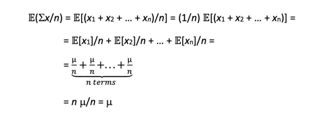
The intricacies of how the mathematical expectation E migrates through the terms are ignored here, but the absence of an assumption about normality (or any distribution for that matter) is crucial. The statistical definition of unbiased is that the expected value of the estimator equals the true value of the population parameter being estimated. In this case, the expected value of the simple mean, the E(Σx/n) term, equals the population value µ, regardless of what µ is or how the data are distributed. This means, according to theory, the sample mean is unbiased for skewed data. A visual explanation is available online.14
The shape of your sample data’s distribution does not affect the shape of your sample mean’s distribution
If you calculate a sample mean of $1,000,000, then how could this vary, why would the variation have a shape, and how would we know the shape in advance? The secret is that your sample mean varies when your sample varies. So, yes, your current sample has a mean of $1,000,000 but you recognize with a different sample you would get different data and a different mean.
Is there anything we can say about all these means we keep calculating from all of the samples we imagine we are taking? Yes, there are two things that researchers have learned. The central location of the mean’s distribution will be at the true mean, and the shape of the mean’s distribution will be “normal.” This second observation, about the mean’s distribution being bell-shaped regardless of the shape of the data’s distribution, is the Central Limit Theorem. A visual explanation is available online.15
References
Le A, Lelli DA, Van Katwyk S, Hogan D, Thavorn K, Tse D. Dizziness at a Canadian tertiary care hospital: a cost-of-illness study. J Otolaryngol Head Neck Surg 2019;48(1):5. https://doi.org/10.1186/s40463-019-0328-9
Salomon L, Gasquet I, Mesbah M, Ravaud P. Construction of a scale measuring inpatients’ opinion on quality of care. Int J Qual Health Care 1999;11:507-16.
https://doi.org/10.1093/intqhc/11.6.507
Gasquet I, Falissard B, Ravaud P. Impact of reminders and method of questionnaire distribution on patient response to mail-back satisfaction survey. J Clin Epidemiol 2001;54:1174-80. https://doi.org/10.1016/s0895-4356(01)00387-0
Moret L, Nguyen JM, Pillet N, Falissard B, Lombrail P, Gasquet I. Improvement of psychometric properties of a scale measuring inpatient satisfaction with care: a better response rate and a reduction of the ceiling effect. BMC Health Serv Res 2007;7:197. https://doi.org/10.1186/1472-6963-7-197
Dyrbye LN, Varkey P, Boone SL, Satele DV, Sloan JA, Shanafelt TD. Physician satisfaction and burnout at different career stages. Mayo Clin Proc 2013;88(12):1358-67.
https://doi.org/10.1016/j.mayocp.2013.07.016
Leigh JP, Kravitz RL, Schembri M, Samuels SJ, Mobley S. Physician career satisfaction across specialties. Arch Intern Med 2002;162(14):1577-84. https://doi.org/10.1001/archinte.162.14.1577
Clark AE, Oswald, AJ, Warr P. Is job satisfaction U-shaped in age? J Occup Organ Psychol 1996;69(1):57-81. https://doi.org/10.1111/j.2044-8325.1996.tb00600.x
Hansen BE. A modern Gauss–Markov theorem. Econometrica 2022;90(3):1283-94. https://doi.org/10.3982/ECTA19255
Kwak SG, Kim JH. Central limit theorem: the cornerstone of modern statistics. Korean J Anesthesiol 2017;70(2):144-156. https://doi.org/10.4097/kjae.2017.70.2.144
Sitch A. Help, my data are skewed: statistical testing for skewed data. BJOG 2020;127(7):812. https://doi.org/10.1111/1471-0528.15571
Briggs A, Nixon R, Dixon S, Thompson S. Parametric modelling of cost data: some simulation evidence. Health Econ 2005;14(4):421-8. https://doi.org/10.1002/hec.941
Hoch JS, O’Reilly RL, Carscadden J. Relationship management therapy for patients with borderline personality disorder. Psychiatr Serv 2006;57(2):179-81. https://doi.org/10.1176/appi.ps.57.2.179
Hoch JS, Haynes SC, Hearney SM, Dewa CS. Analyzing a cost-effectiveness dataset: a speech and language example for clinicians. Semin Speech Lang 2022;43(3):244-54. https://doi.org/10.1055/s-0042-1750347
SahilKadu96. Sample mean is an unbiased estimator of population mean. Blog post. Medium; 2025. https://tinyurl.com/bdhf7ztk
Data Science Delight. Central limit theorem: a beginner’s guide. Blog post. Medium; 2024Accessed September 20, 2026: https://tinyurl.com/4r76bntj
Authors
Jeffrey S. Hoch, MA, PhD, is a professor in the Department of Public Health Sciences at the University of California Davis (UC Davis). He is chief of the Division of Health Policy and Management and associate director of the Center for Healthcare Policy and Research at UC Davis.
Carolyn S. Dewa, MPH, PhD, is a professor in the Department of Psychiatry and Behavioral Sciences and the Department of Public Health Sciences at UC Davis.
Correspondence to:
jshoch@health.ucdavis.edu