
HEALTH ECONOMICS
Same but different: new options that are not significantly different can be cost-effective

Jeffrey S. Hoch, PhD,
Carolyn S. Dewa, MPH, PhD
In this eighth article in the health economics series, we explore the idea that a new treatment can be cost-effective but not significantly different from usual care in terms of costs or outcomes. This situation occurs because a cost-effectiveness analysis considers costs and outcomes simultaneously. In addition, researchers often employ a different statistical approach, using a Bayesian instead of frequentist framework. We provide an example illustrating a new option with non-statistically significant differences in both cost and health outcome with a high probability of cost-effectiveness.
KEY WORDS: leadership, cost-effectiveness analysis, health economics
Hoch JS, Dewa CS. Same but different: new treatments that are not significantly different can be cost-effective. Can J Physician Leadersh 12(2): 114-121. https://doi.org/10.37964/cr24810
It is easy to think of cost-effectiveness analysis (CEA) as a study that tests both cost and effectiveness for statistical significance. Often researchers design clinical trials to detect a statistical difference in the main outcome (e.g., treatment effectiveness), potentially leaving the test of cost differences underpowered. Raftery and colleagues1 studied the prevalence of “paradoxical conclusions” in “doubly null” trials with non-statistically significant differences in both cost and health outcome. They found that almost 40% of trials they reviewed had doubly null results and about a third drew economic conclusions in favour of a new option. That is, the new treatment was neither cheaper nor more effective. Yet, researchers concluded it was cost-effective. How could this be?
In this article, we explore conditions under which such a seemingly paradoxical conclusion can arise. Different interpretations of uncertainty (e.g., Bayesian vs. frequentist) explain the important distinction that can help readers appreciate “probability of cost-effectiveness” as opposed to “statistical significance.”
Reviewing cost-effectiveness analysis
We briefly review CEA in this section, as previous articles in the health economics series have discussed it in greater detail.2-7 CEA produces estimates of extra cost (ΔC) and extra health outcome, viewed as extra effect (ΔE). To illustrate the main concepts, we create hypothetical data with descriptive results.
Table 1: Results from a hypothetical study
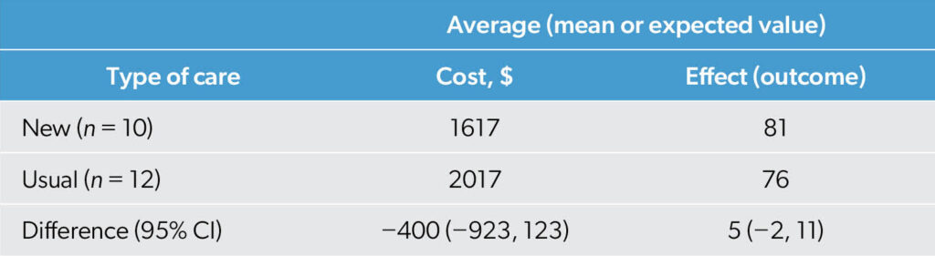
Table 1 shows that a new type of care is both cheaper (ΔC = −$400) and more effective (ΔE = 5). However, as the confidence intervals for both ΔC (−923, 123) and ΔE (−2, 11) include 0, neither the cost-saving estimate nor the effectiveness estimate is precise enough to rule out a hypothesis of no difference. The new option may be more costly or less costly; it may be more effective or less effective. This might be expected given that the hypothetical data are based on only 22 people. So, what are we to conclude about a small study showing a promising value proposition? The signal is there but the noise is loud. What tools can be used to make CEA meaningful for decision-makers?
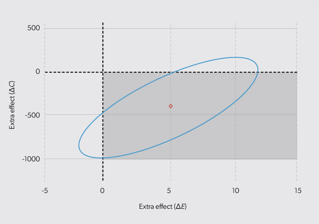
Figure 1: Cost-effectiveness plane showing both an estimate and uncertainty.
Conveying CEA information
Researchers often use two related figures to convey cost-effectiveness conclusions. The first is a cost-effectiveness plane showing both an estimate and uncertainty.
Note: The estimate is shown as ◊, with 95% confidence interval for ΔC and ΔE illustrated by the ellipse. The shaded area shows where there is more effectiveness and less cost.
Using data from Table 1, Figure 1 shows that the estimate (i.e., ◊) for the new option is both cheaper (ΔC < 0) and more effective (ΔE > 0). The exact location of the estimate is at (5, −400), corresponding to the mean results in Table 1. Uncertainty is conveyed by the ellipse, which serves as a 95% confidence interval (CI) for the estimate. Assuming the means are jointly normally distributed with cost and effect correlated implies an ellipse-shaped 95% CI.8
Treating cost and effect as two separate outcomes would create a 95% CI shaped like a rectangular box.9
The 95% CI ellipse shows it is possible for ΔC or ΔE or both to be zero. In fact, the current evidence shows that the new option may be:
- cheaper and less effective
- cheaper and more effective
- more expensive and more effective
However, the bulk of the ellipse’s area is in the “saves money and is more effective” region. This means this is the most likely scenario (with the highest probability). Consequently, analysts should more confidently conclude that the new option is a good deal.
What is a good deal?
For some decision-makers a good deal means saving money (i.e., ΔC < 0); for others, good means better health outcome (i.e., ΔE > 0). Often, leaders must be nuanced in their approach to value and consider when the extra effect is worth the extra cost. Health economists use “cost-effectiveness threshold” to refer to the point where the extra effect is exactly worth the extra cost. Some have speculated that the cost-effectiveness threshold could be a single number or a range.10-12 Suffice it to say, the person doing the analysis for you does not know the number you want to use for the cost-effectiveness threshold in your context. Consequently, rigorous research provides a wide range of values for your consideration.
Figure 2: Cost-effectiveness plane with different cost-effectiveness thresholds.
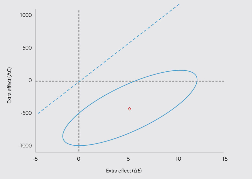
Note: The estimate is shown as ◊, with 95% confidence interval for ΔE and ΔC illustrated by the ellipse. The dashed lines represent three cost effectiveness thresholds.
Figure 2 illustrates the application of three cost-effectiveness thresholds (dashed lines showing ΔC/ΔE) to the results in Figure 1. The horizontal dashed line illustrates a cost-effectiveness threshold of zero. This is consistent with the thinking that the only good deal is one where the new option saves money (i.e., ΔC < 0). In this setting, anything below the horizontal line represents good value for money (regardless of the effectiveness!). The vertical dashed line illustrates a cost-effectiveness threshold of infinity. Anything to the right of the line represents a good deal (regardless of the cost!). If you are like most decision-makers, you probably have a cost-effectiveness threshold somewhere between 0 and infinity. The grey dashed line in Figure 2 has a slope of 100. On this line, each unit of extra effect is worth $100. Anything below this dashed line is considered cost-effective, including options that are more expensive (and more effective) as well as those that are less effective (and less costly).
In Figure 2, the cost-effectiveness estimate (◊) falls below each of the cost-effectiveness threshold lines. This means that the new option is cost-effective, regardless of the decision-maker’s cost-effectiveness threshold. However, the probability that the new option is cost-effective varies with the cost-effectiveness threshold. This is evident when examining the relation between each cost-effectiveness threshold and the 95% confidence ellipse. The dark dashed lines cut through the upper and lower parts of the ellipse, while the grey dashed line does not intersect the ellipse. By keeping track of how much of the uncertainty is below the dashed lines, researchers can report the probability of cost-effectiveness. We can use a cost-effectiveness acceptability curve (CEAC) to display the probability of cost-effectiveness for each value of the cost-effectiveness threshold.
The probability of cost-effectiveness
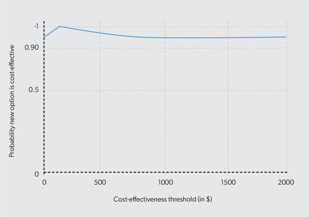
On the CEAC in Figure 3,8 probability ranges from 94% to 100%. The horizontal axis shows values corresponding to the slopes of the dashed lines (representing cost effectiveness thresholds) in Figure 2. The vertical axis of Figure 3 shows the probability that the new option is cost-effective, which corresponds to the proportion of probability that is below the dashed lines in Figure 2. The horizontal axis shows the cost-effectiveness threshold from $0 to $2000. Figure 3 shows that the probability of cost-effectiveness is very high and does not vary much.
Figure 3: Cost-effectiveness acceptability curve for a range of cost-effectiveness thresholds.
The concept of “probability of cost-effectiveness” uses a Bayesian interpretation of uncertainty, instead of a traditional frequentist interpretation of probability (p). The value of Figure 3’s vertical axis is not changed by this switch in paradigm, but the interpretation is. Because the Bayesian interpretation is more intuitive, it has been widely adopted in the cost-effectiveness literature. One can convert a p-value into “probability of cost-effectiveness” and then use this for the vertical axis of the cost-effectiveness acceptability curve (see Figure 3).13
Discussion
The data in Table 1 provide an example of a new option that is less costly (i.e., ΔC < 0) and more effective (i.e., ΔE > 0) than usual care. However, when looked at separately, neither estimate of the difference in cost and effectiveness is statistically significant. Studying the cost and effect outcomes simultaneously produces a 95% confidence interval shown as the ellipse in Figure 1. Because the ellipse stretches into three quadrants in Figure 2, the promising estimate of less cost and more effect could have occurred by chance alone. Clear from Figure 2 is that most of the time, most of the ellipse is below the cost-effectiveness threshold lines; there is a high probability that the new option is cost-effective, even though it does not have statistically significant cost or effect differences. This is because most of the ellipse is in the southeast quadrant of Figure 2 meaning there is high probability that the new option is both more effective and less costly.
Figure 3 demonstrates that it is possible for the probability of cost-effectiveness to increase and then decrease as the assumed cost-effectiveness threshold value changes. This change in slope is related to the change in probability that is below Figure 2’s dashed line. The mostly flat line in Figure 3 vacillating between 94% and 100% means that the new option has a very high probability of cost-effectiveness for all cost-effectiveness threshold values considered in the analysis.
The example reminds us of the difference between statistical uncertainty and decision uncertainty. The large ellipse shows a lot of statistical uncertainty. So much in fact, it is not clear whether the new option compared to usual care is more or less costly or whether it is more or less effective. The high statistical uncertainty is due to the small sample size. However, the decision uncertainty is modest. Most of the probability characterizing the uncertainty can be classified as a good deal (below the cost-effectiveness threshold line, regardless of which one is chosen).
Leaders interested in using the results from economic evaluations, such as CEA, should rely on viewing both the estimate and its uncertainty to help inform their decisions. In this process, it is important to separate uncertainty of interest to the analyst (size of the ellipse) from uncertainty of interest to the decision-maker (location of the ellipse). Whether the ellipse spills over into multiple quadrants is important, but so is its relation to different assumed cost-effectiveness thresholds (the dashed lines). This means that it is important to understand the cost-effectiveness thresholds that analysts assume and whether they fit with your context. Since these thresholds are unknown to the analyst, research should employ a variety of them for decision-makers to consider.
References
Raftery J, Williams HC, Clarke A, Thornton J, Norrie J, Snooks H, et al. “Not clinically effective but cost-effective“ — paradoxical conclusions in randomised controlled trials with “doubly null“ results: a cross-sectional study. BMJ Open 2020;10(1):e029596. https://doi.org/10.1136/bmjopen-2019-029596
Hoch J, Dewa C. The occult of efficiency: frank, and Stein’s, advice for physician leaders. Can J Physician Leadersh 2024;10(1):29-32. https://doi.org/10.37964/cr24780
Hoch J, Dewa C. Cost is not a four-letter word: focus on what you can change. Can J Physician Leadersh 2024;10(2):64-8. https://doi.org/10.37964/cr24783
Hoch J, Dewa C. Maximizing success when it is the product of two things that go in opposition directions: the magic of elasticity. Can J Physician Leadersh 2024;10(3):84-91. https://doi.org/10.37964/cr24784
Hoch J, Dewa C. Cost-minimization analysis: showing something is cheaper does not necessarily show that it is better. Can J Physician Leadersh 2025;11(1):31-9.
https://doi.org/10.37964/cr24789
Hoch J, Dewa C. Choosing one from many: efficiency in a multi-option world. Can J Physician Leadersh 2025;11(2):102-8. https://doi.org/10.37964/cr24793
Hoch J, Dewa C. Analyzing cost-effectiveness data: from calculation to illustration. Can J Physician Leadersh 2025;11(3):143-51. https://doi.org/10.37964/cr24798
Van Hout BA, Al MJ, Gordon GS, Rutten FF. Costs, effects and C/E-ratios alongside a clinical trial. Health Econ 1994;3(5):309-19. https://doi.org/10.1002/hec.4730030505
O’Brien BJ, Drummond MF, Labelle RJ, William A. In search of power and significance: issues in the design and analysis of stochastic cost-effectiveness studies in health care. Med Care 1994;32(2):150-63. https://doi.org/10.1097/00005650-199402000-00006
Laupacis A, Feeny D, Detsky AS, Tugwell PX. How attractive does a new technology have to be to warrant adoption and utilization? Tentative guidelines for using clinical and economic evaluations. CMAJ 1992;146(4):473-81. https://pmc.ncbi.nlm.nih.gov/articles/PMC1488412/
Naylor CD, Williams JI, Basinski A, Goel V. Technology assessment and cost-effectiveness analysis: misguided guidelines? CMAJ 1993;148(6):921-4. https://pmc.ncbi.nlm.nih.gov/articles/PMC1490754/
Grosse SD. Assessing cost-effectiveness in healthcare: history of the $50,000 per QALY threshold. Expert Rev Pharmacoecon Outcomes Res 2008;8(2):165-78.
https://doi.org/10.1586/14737167.8.2.165
Hoch JS, Rockx MA, Krahn AD. Using the net benefit regression framework to construct cost-effectiveness acceptability curves: an example using data from a trial of external loop recorders versus Holter monitoring for ambulatory monitoring of “community acquired” syncope. BMC Health Serv Res 2006;6:68. https://doi.org/10.1186/1472-6963-6-68
Authors
Jeffrey S. Hoch, MA, PhD, is a professor in the Department of Public Health Sciences at the University of California Davis (UC Davis). He is chief of the Division of Health Policy and Management and associate director of the Center for Healthcare Policy and Research at UC Davis.
Carolyn S. Dewa, MPH, PhD, is a professor in the Department of Psychiatry and Behavioral Sciences and the Department of Public Health Sciences at UC Davis.
Correspondence to: jshoch@health.ucdavis.edu